
Areas by Computer
Mark Fineman
Have a home computer? Looking for a way to calculate areas of complex shapes? Read on.
Anyone who has ever designed a model airplane knows that such a craft is in many ways a collection of decisions and compromises: What is the best airfoil? What are the best nose and tail moments? What shape should be used for the wing and tail? The list can be a long one.
While to some extent special design considerations enter into the creation of any type of flying model, the category of rubber-scale airplanes presents the designer with his biggest challenges. By their very nature, it is sometimes surprising that such models fly at all, for they are not entirely governed by the same principles that dictate their full-size counterparts' flight. The point is best illustrated in the case of wing and tail areas.
Generally speaking, slow-flying scale models require proportionally larger stabilizers than the full-size airplanes they represent. The exact stabilizer area, expressed as a percentage of wing area, is affected by several variables, including the tail moment, speed of the aircraft, and whether or not the incidence of the stabilizer can be adjusted in flight.
Many designers, myself included, factor in a subjective, aesthetic variable as well, since a grossly enlarged stabilizer may look just plain ridiculous. As a matter of practical experience, the smallest stabilizer that I have ever successfully flown was on a Mr. Smoothie racer at 17% of wing area. It is more usual for the stabilizer area to be somewhere between 25% and 30% of the wing area. This figure is somewhat smaller than the 33 1/3% given as a standard for nonscale, rubber-powered models—again, for reasons of appearance.
Calculating areas
I have always found the standard techniques for calculating areas to be laborious. In times past, this was done by drawing the wing or stabilizer outline onto quadrille graph paper and then counting all the little boxes (and fractions of boxes) contained within the outline. The total number of quarter-inch squares was then converted into square inches. As I said, laborious.
So hated was this procedure that I even tried pouring BBs into a bounded wing shape in order to see how many square inches of graph paper they would occupy. That method, as you can imagine, was even worse.
When I ran across a procedure in BYTE magazine (February 1987; authored by Stolk and Ettersahn) that could calculate the areas of irregular shapes, it seemed a natural for the wing and stabilizer area problem. When incorporated into a simple program, the technique neatly does the job, and without digitizing tablets or other expensive computer accessories. In fact, the procedure is so simple, and the program so unsophisticated, that it can be adapted to virtually any home computer, even the simplest.
Computer Area/Fineman
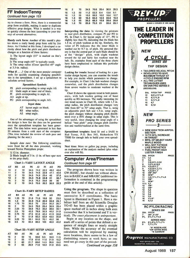
The program shown here was written in GW-BASIC, but should run without alteration in BASICA and MBASIC (additional information is contained in the programming guide at the end of this article).
Using the program
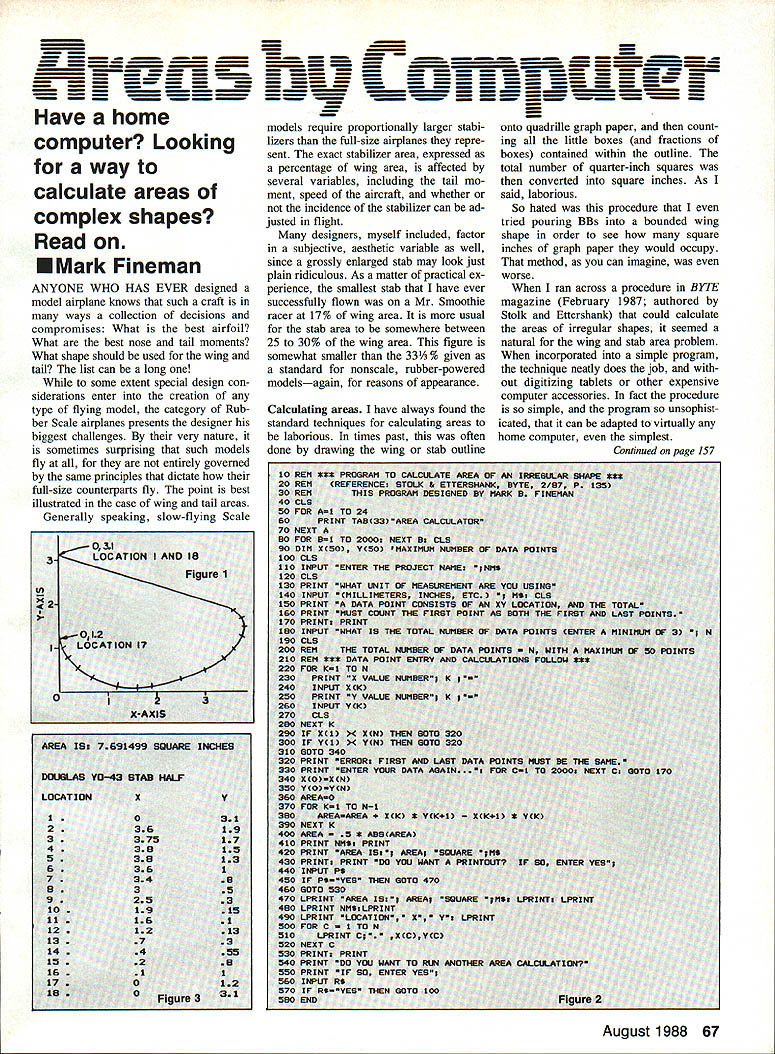
The shape in question must first be described as a collection of successive X–Y coordinates. The basic layout is illustrated in Figure 1. Here a stabilizer half from an old Scientific Douglas YO-43 has been placed within a graphic space marked off in inches along both axes (remember that X is horizontal and Y is vertical). The exact placement is unimportant.
Begin at any location on the shape, and mark off a series of points that delimit a sequence of straight lines or nearly straight lines. While the accuracy of the eventual calculation will be improved by adding more points, there is a law of diminishing returns at work; you need not go crazy in this part of the procedure.
The program allows a maximum of 50 locations per program run, which should be more than enough. Each location is then assigned a horizontal (X) and vertical (Y) value. The easiest and quickest way to do this is to draw the shape on tracing paper and place the tracing on top of graph paper that is ruled in millimeters or tenths of an inch. For clarity, the inch subdivisions are not shown in Figure 1, but they were used in the original plot.
The stabilizer outline in Figure 1 might well have been somewhat smaller, since one would normally only plot that part of the flying surface that actually accounts for lift, not the area contained within the fuselage. I have found that it takes relatively little time to plot X–Y coordinates—just a few minutes, even for curved surfaces.
Once the X–Y locations have been determined, run the program and enter the coordinates. Note that the program first asks for the total number of locations, and that the first X–Y location is included twice, once as the first location and then again as the last. This is illustrated in Figure 1. The program includes an error trap to ensure that you have followed this convention. If you don't, the program will exit and make you re-enter all the data. Take your time entering the coordinates, checking along the way to avoid typing errors.
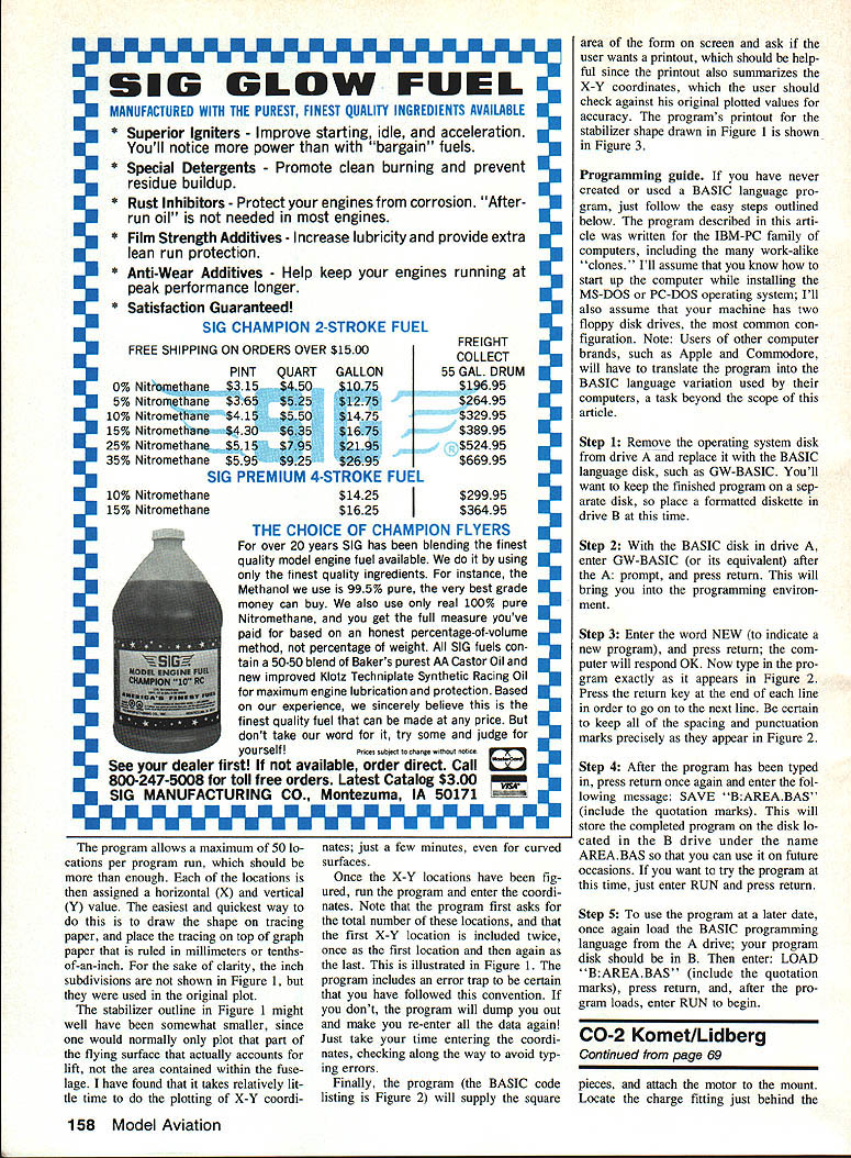
Finally, the program (the BASIC code listing is Figure 2) will display the area in square inches on screen and ask if you want a printout. The printout is helpful because it also summarizes the X–Y coordinates, which you should check against your original plotted values for accuracy. The program's printout for the stabilizer shape drawn in Figure 1 is shown in Figure 3.
Programming guide
If you have never created or used a BASIC language program, follow the easy steps outlined below. The program described in this article was written for the IBM‑PC family of computers, including the many work‑alike "clones." I'll assume that you know how to start up the computer while running MS‑DOS or PC‑DOS; I'll also assume that your machine has two floppy disk drives, the most common configuration.
Note: Users of other computer brands, such as Apple and Commodore, will have to translate the program into the BASIC language native to their computers, a task beyond the scope of this article.
- Remove the operating system disk from drive A and replace it with the BASIC language disk, such as GW‑BASIC. You'll want to keep the finished program on a separate disk, so place a formatted diskette in drive B at this time.
- With the BASIC disk in drive A, enter GW‑BASIC (or its equivalent) after the A: prompt, and press Return. This will bring you into the programming environment.
- Enter the word NEW (to indicate a new program), and press Return; the computer will respond OK. Now type in the program exactly as it appears in Figure 2. Press the Return key at the end of each line to go on to the next line. Be certain to keep all spacing and punctuation precisely as they appear in Figure 2.
- After the program has been typed in, press Return once again and enter the following command: SAVE "B:AREA.BAS" (include the quotation marks). This will store the completed program on the disk in drive B under the name AREA.BAS so that you can use it on future occasions. If you want to try the program at this time, just enter RUN and press Return.
- To use the program at a later date, once again load the BASIC programming language from the A drive; your program disk should be in B. Then enter: LOAD "B:AREA.BAS" (include the quotation marks), press Return, and after the program loads, enter RUN to begin.
Transcribed from original scans by AI. Minor OCR errors may remain.

