
Scaling Laws
by Dave Harding
At our flying field a while ago I met a prospective member who was waiting for one of our instructors to have a session with his 40-size trainer on dual control. He explained that this was his second model; the first was destroyed when he flew it through a tree.
While waiting, he watched two club members flying their electric park flyers, and a funny look appeared on his face. He realized that he could be learning the basics of flight control on a much smaller, less-expensive airplane—one that flew slowly enough to allow errors and recovery without the expense involved in making the same mistakes on the conventional trainer. One of the park flyers was also learning—and doing it solo. He made repeated dunks into the long grass beyond our runway. Each time the result was his picking up the model, adjusting the wing, and launching again for another flight. How could that be? The bigger airplane would almost be destroyed with such handling. What was going on?
Scaling laws. Among all of the wonderful laws of physics that bind our universe are sets of principles known as scaling laws. These are the relationships that define the effects that size have on physical behavior. They are fundamental to our hobby and to our everyday lives.
The primary set of scaling laws of interest to us are sometimes known as “square-cube” laws, and their first part relates to how an object’s surface area and volume vary with its size.
Area, Volume, and Weight
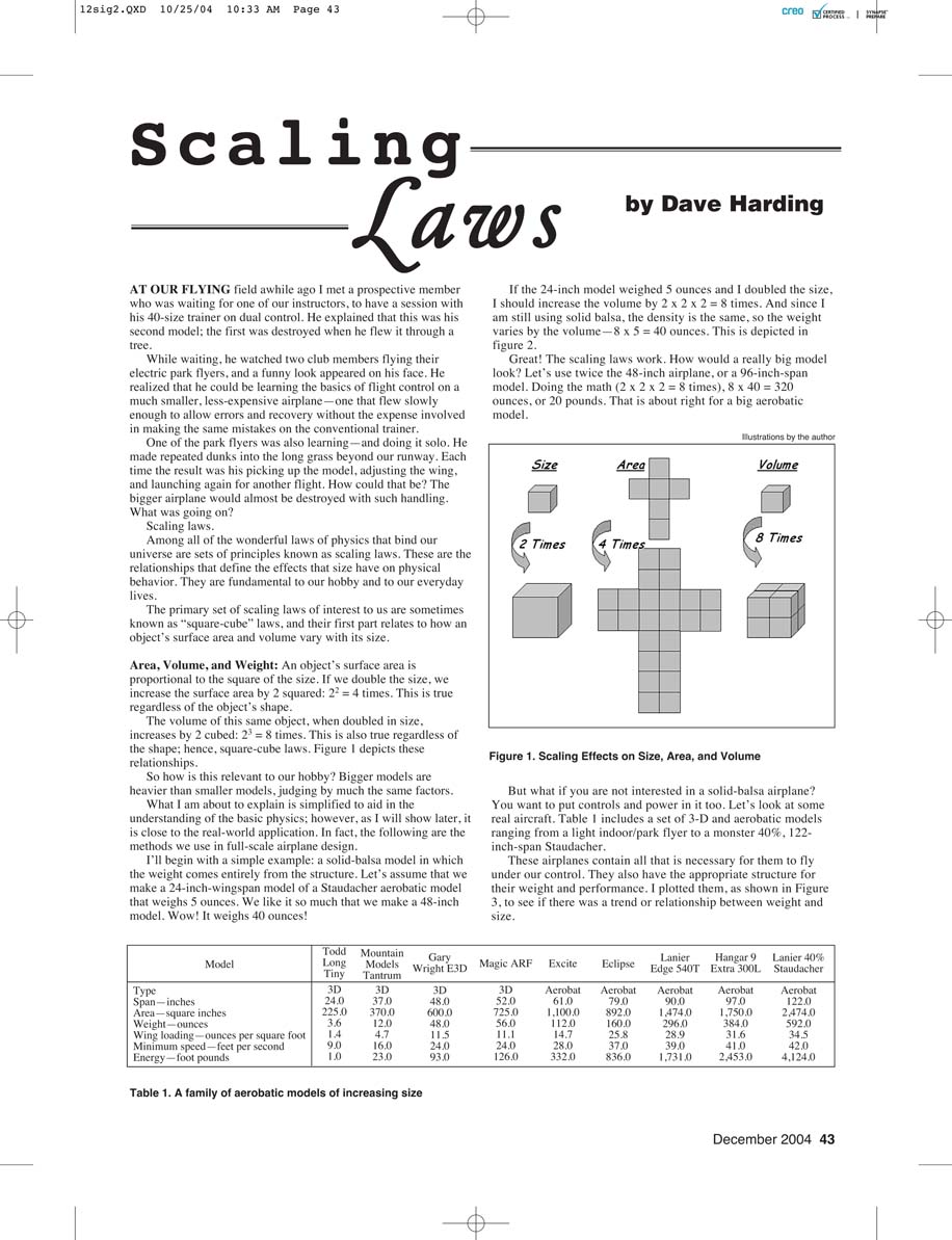
An object’s surface area is proportional to the square of the size. If we double the size, we increase the surface area by 2^2 = 4 times. This is true regardless of the object’s shape.
The volume of this same object, when doubled in size, increases by 2^3 = 8 times. This is also true regardless of the shape; hence, square-cube laws.
So how is this relevant to our hobby? Bigger models are heavier than smaller models, judged by much the same factors.
What I am about to explain is simplified to aid in the understanding of the basic physics; however, as I will show later, it is close to real-world application. In fact, the following are the methods we use in full-scale airplane design.
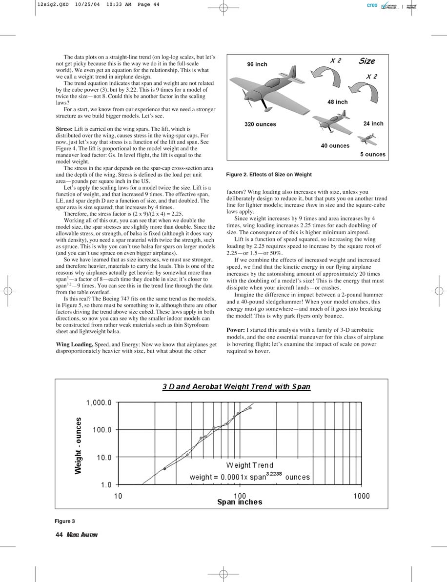
I’ll begin with a simple example: a solid-balsa model in which the weight comes entirely from the structure. Let’s assume that we make a 24-inch-wingspan model of a Staudacher aerobatic model that weighs 5 ounces. We like it so much that we make a 48-inch model. Wow! It weighs 40 ounces!
If the 24-inch model weighed 5 ounces and I doubled the size, I should increase the volume by 2 × 2 × 2 = 8 times. And since I am still using solid balsa, the density is the same, so the weight varies by the volume—8 × 5 = 40 ounces. This is depicted in figure 2.
Great! The scaling laws work. How would a really big model look? Let’s use twice the 48-inch airplane, or a 96-inch-span model. Doing the math (2 × 2 × 2 = 8 times), 8 × 40 = 320 ounces, or 20 pounds. That is about right for a big aerobatic model.
But what if you are not interested in a solid-balsa airplane? You want to put controls and power in it too. Let’s look at some real aircraft. Table 1 includes a set of 3-D and aerobatic models ranging from a light indoor/park flyer to a monster 40%, 122-inch-span Staudacher.
These airplanes contain all that is necessary for them to fly under our control. They also have the appropriate structure for their weight and performance. I plotted them, as shown in Figure 3, to see if there was a trend or relationship between weight and size.
The data plots on a straight-line trend (on log-log scales, but let's not get picky because this is the way we do it in the full-scale world). We even get an equation for the relationship. This is what we call a weight trend in airplane design.
The trend equation indicates that span and weight are not related by the cube power (3), but by 3.22. This is 9 times for a model of twice the size—not 8. Could this be another factor in the scaling laws?
For a start, we know from our experience that we need a stronger structure as we build bigger models. Let's see.
Stress
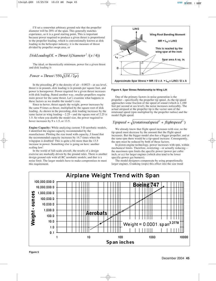
Lift is carried on the wing spars. The lift, which is distributed over the wing, causes stress in the wing-spar caps. For now, just let's say that stress is a function of the lift and span. See Figure 4. The lift is proportional to the model weight and the maneuver load factor: G's. In level flight, the lift is equal to the model weight.
The stress in the spar depends on the spar-cap cross-sectional area and the depth of the wing. Stress is defined as the load per unit area—pounds per square inch in the US.
Let's apply the scaling laws for a model twice the size. Lift is a function of weight, and that increased 9 times. The effective span, LE, and spar depth D are a function of size, and those doubled. The spar area is size squared; that increases by 4 times.
Therefore, the stress factor is (2 × 9) / (2 × 4) = 2.25.
Working all of this out, you can see that when we double the model size, the spar stresses are slightly more than double. Since the allowable stress, or strength, of balsa is fixed (although it does vary with density), you need a spar material with little change in strength, such as spruce. This is why you can't use balsa for spars on larger models (and you can't use spruce on even bigger airplanes).
So we have learned that as size increases, we must use stronger, and therefore heavier, materials to carry the loads. This is one of the reasons why airplanes actually get heavier by somewhat more than span^3—a factor of 8—each time they double in size; it's closer to span^3.22—9 times. You can see this in the trend line through the data from the table overview.
Is this real? The Boeing 747 fits on the same trend as the models, in Figure 5, so there must be something to it, although there are other factors driving the trend above size cube. These laws apply in both directions, so now you can see why the smaller indoor models can be constructed from lighter raw materials such as thin Styrofoam sheet and lightweight balsa.
Wing Loading, Speed, and Energy
Now we know that airplanes get disproportionately heavier with size, but what about the other factors? Wing loading also increases with size, unless you deliberately design to reduce it, but that puts you on another trend line for lighter models; increase them in size and the square-cube laws apply.
Since weight increases by 9 times and area increases by 4 times, wing loading increases 2.25 times for each doubling of size. The consequence of this is higher minimum airspeed.
Lift is a function of speed squared, so increasing the wing loading by 2.25 requires speed to increase by the square root of 2.25—or 1.5—or 50%.
If we combine the effects of increased weight and increased speed, we find that the kinetic energy in our flying airplane increases by the astonishing amount of approximately 20 times with the doubling of a model's size! This is the energy that must be dissipated when your aircraft lands—or crashes.
Imagine the difference in impact between a 2-pound hammer and a 40-pound sledgehammer. When your model crashes, this energy must go somewhere—and much of it goes into breaking the model! This is why park flyers only bounce.
Power
I started this analysis with a family of 3-D aerobatic models, and the one essential maneuver for this class of airplane is hovering flight; let's examine the impact of scale on power required to hover.
I'll set a somewhat arbitrary ground rule that the propeller diameter will be 20% of the span. This generally matches experience, so it is a good starting point. This is important because power required to produce a given thrust is proportional to the propeller loading, which is conventionally known as disk loading in the helicopter industry; it is the measure of thrust divided by propeller swept area, or
- Disk Loading DL = Thrust / (pi × Diameter^2 / 4)
The ideal, or theoretically minimum, power for a given thrust and disk loading is
- Power = (Thrust × sqrt(DL / (2 × rho))) / 550
In the preceding, rho is the density of air — 0.0023 slugs/ft^3 at sea level, thrust is in pounds, disk loading is in pounds per square foot, and power is in horsepower. Power required for a given thrust increases with disk loading. Stated another way, smaller propellers require more power for the same thrust. Let's examine what happens to these factors as we double the model's size.
Since to hover, thrust equals the weight, power increases by the same 9 times as thrust, multiplied by the square root of disk loading. As shown above, disk loading increases by the same factor as wing loading — 2.25 — and the square root of 2.25 is 1.5. So when you double the model size, the power required to hover increases by 9 × 1.5 = 13.5.
Engine Capacity
While analyzing current 3-D aerobatic models, I identified the engine capacity recommended by the manufacturer. Plotting the size trend with capacity, I found that the recommended capacity increases by 14.7 times when the wingspan is doubled! This is quite a bit more than the 13.5 increase in power. Something else is going on here: another scaling law!
In the world of full-scale aircraft, the results of a design exercise are markedly driven by the ground rules. There is another design ground rule with all RC aerobatic models, and that is a noise limit. The larger models have to make compromises to meet this requirement.
One of the primary factors in noise generation is the propeller—specifically the propeller tip speed. As the tip speed approaches some fraction of the speed of sound (which is about 1,100 feet per second at sea level), the noise increases noticeably. The actual airspeed at the propeller tip is the vector sum of the rotational speed (rpm multiplied by the propeller radius) and the model flight speed:
- Tipspeed = sqrt(rotationalspeed^2 + flightspeed^2)
We already know that flight speed increases with size, so the tip speed must decrease by the amount that the flight speed increases. But the bigger model also has a bigger propeller, and at the same rpm there would be a tip-speed increase. Consequently, the rpm must be reduced by both of these factors.
In piston-engine technology, power increases with rpm, within mechanical limits. Therefore, restricting — or actually reducing — the maximum rpm limits the specific power (power per cubic inch, or cc) for larger engines (which also tend to be lower specific-power gas burners). The model designers compensate by using proportionally larger engines. Cranking this effect into the size trend results in the required capacity increasing by the higher 14.7 times for a double-size model.
Maximum Speed
You have seen that the scaling laws drive us to disproportionately more power as we increase the model size, so it should be no surprise that this power increase allows the larger model to go faster.
The typical RC model's theoretical maximum speed is set by power and aerodynamic drag. For our "overpowered" models, the drag at maximum speed is predominantly from wetted area, skin friction, and form factor, or streamlining.
We conventionally express this drag in terms of the drag coefficient, or Cd. Drag is related to Cd by a reference area. Multiplying the Cd by the reference area and multiplying that by the dynamic pressure calculates the drag. It looks like the following formula, where the units are pounds, feet, and feet per second.
- Drag = 0.0012 × V^2 × A × Cd
For an airplane, the reference area—A—is conventionally the wing area. Notice that area multiplied by Cd is also an area.
This is sometimes called the "equivalent flat plate drag area," because a flat plate with this area, placed perpendicular to the airstream, would produce roughly the same drag.
Using this concept allows you to estimate the effects of design changes such as retracting the landing gear, where you would subtract an area equivalent to the landing-gear frontal area from the initial equivalent flat plate drag area.
For a given geometry, Cd remains constant with size changes (excepting the effects defined by that other scaling law discovered by the good Doctor Reynolds, but we will ignore this for now).
For a given power and drag we can calculate the airspeed using the following formula, where V is in feet per second and drag is in pounds.
- V = 550 × Power / Drag
Substituting the preceding formula for drag, we get the following, where A is in square feet.
- Speed V = 77 × (Power / (A × Cd))^(1/3)
Now you can estimate the effect of doubling size on maximum speed. When you double the size of the model, the wing area—and therefore the drag area—increases by 4 times. From my prior investigation where I doubled the size, the power increased by 13.5 times. Now you see that the speed increase will be proportional to the cube root of 13.5/4. The speed-increase factor will be:
- (13.5 / 4)^(1/3) = (3.375)^(1/3) = 1.5
So when size increases by a factor of 2, the theoretical maximum speed increases by a factor of 1.5, which is 50%. I have called this speed increase "theoretical" because in practice there is another limiting factor: the propeller. In an aerobatic model, particularly one that is geared toward 3-D maneuvers, you select a propeller that is aimed at maximizing the hover and low-speed performance.
Propellers only work well in a narrow speed range. Hover propellers don't work at speed. However, if we changed the propeller for one that optimizes at the maximum speed—specifically one with the correct smaller diameter and higher pitch—we should be able to come close to demonstrating the speed prediction. But propellers are a subject for another time.
Table 2 — Summary of Scale Effects (doubling size)
- Surface Area / Wing Area: Multiplier = 4 ; Exponent y = 2
- Volume: Multiplier = 8 ; Exponent y = 3
- Weight: Multiplier = 9 ; Exponent y = 3.22
- Wing Loading: Multiplier = 2.25 ; Exponent y = 1.22
- Minimum Speed: Multiplier = 1.5 ; Exponent y = 0.61
- Kinetic Energy at Minimum Speed: Multiplier = 20.25 ; Exponent y = 4.4
- Power Required: Multiplier = 13.5 ; Exponent y = 3.8
- Potential Maximum Speed: Multiplier = 1.5 ; Exponent y = 0.61
To calculate for a specific scale using a scientific calculator, first calculate the scale factor as the fraction (new span / baseline span). Second, raise that number to the exponent shown by pressing the x^y button then the exponent from the table. The result is the scaling factor you use to multiply the parameter from your baseline model.
Applying these factors to the 24-inch, 5-ounce balsa Staudacher and estimating the weight of a 96-inch model:
- Weight = 5 × (96 / 24)^3.22 = 5 × 4^3.22 = 5 × 86.8 = 434 ounces = 27 pounds (approx.)
Happy scaling.
MA
Dave Harding 4948 Jefferson Dr. Brookhaven, PA 19015
Transcribed from original scans by AI. Minor OCR errors may remain.

